Using Flurry Data to Compare App Retention Strategies in R

Eric Fram

All of the code used here is available on GitHub

##Introduction

This document will show you how to use R to compare app retention data downloaded from Flurry. The code here accompanies the article I published on ZippyBrain.com titled “Do Local Notifications Increase Retention Rates?”. Link to the Article

Here, I compare retention data between two different apps, but you can also use this code to compare data between different versions of the same app or between different date ranges of the same app.

The sample .csv files included in this repository are formatted exactly the same as any retention data files you download from Flurry.

##Reading and Processing the Data

First, I initialize 5 variables for the directory my files are stored in, the names of the two .csv files with the retention data, and the names of the two apps, app versions, or app date ranges I am comparing. Here, I’m using the sample data, but you will need to modify these if you are using your own data.

directory <- paste(getwd())
app1.filename <- 'Beehive-ReturnRate_Sample.csv'
app2.filename <- 'Birdhouse-ReturnRate_Sample.csv'
app1.name <- "Beehive"
app2.name <- "Birdhouse"

Next I read the data from these files into R. The .csv files that come from Flurry have extraneous information and are not formatted for use in R, so I make some adjustments to the files after reading them in. The getData function here does the following:

1. Read the .csv file into R, skipping the first row and the first 2 columns (which contain header labels, date, and cohort size)
2. Take one the first row, which is days since install, and the last row, which is the overall return rate for each day
3. Transpose the data frame
4. Add the correct app name to observation
5. Label columns properly

#read the .csv files as they arrive from Flurry, then convert them to raw data
getData <- function(directory,app.filename,app.name) {
      
      #read the .csv file | skip 1 row and 2 columns
      df <- read.csv(paste(directory,'/',app.filename,sep=""),skip=1,
                     colClasses=c("NULL","NULL",rep('character',29)),header=FALSE)
      
      #select only the first and last rows ("Days Since Install" and "Return Rate")
      df <- df[c(1,nrow(df)),]
      
      #transpose data frame
      df <- as.data.frame(t(df))
      
      #ditch "row.names" column, name columns properly, and fill in app name
      df$app <- app.name
      colnames(df)[1:2] <- c("daysSinceInstall","returnRate")
      df
}

#run the getData function for both apps
app1.data <- getData(directory,app1.filename,app1.name)
app2.data <- getData(directory,app2.filename,app2.name)

The next step is to combine the information from both files into one files and to correct the column classes.

#combine data from both apps into one data frame and drop old dataframes
both.data <- rbind(app1.data,app2.data)
rm(app1.data)
rm(app2.data)

#fix percents and set correct column classes
both.data$returnRate <- as.numeric(as.character((gsub("%","",both.data$returnRate))))/100
both.data$daysSinceInstall <- as.numeric(as.character(both.data$daysSinceInstall))

#Plotting and Analyzing the Data

At this point, the data is ready to plot. I use ggplot2 for this.

#plot the return rates
require(ggplot2)
plot <- ggplot(data=both.data,aes(x=both.data$daysSinceInstall,y=both.data$returnRate,group=app,color=app))
plot <- plot + geom_line(stat='identity',size=1)
plot <- plot + xlab("Days Since Install") + ylab("Return Rate")
plot <- plot + geom_point() +  scale_colour_discrete(name  = 'App')
plot <- plot + scale_x_continuous(breaks=seq(0, 30, 1))
plot <- plot + scale_y_continuous(breaks=seq(0,.3,.01))
plot

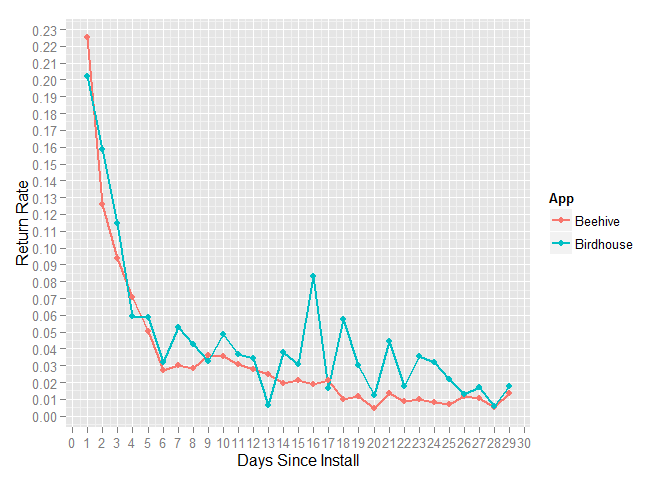
Using this sample data, it looks like Birdhouse is somewhat better at retaining users than Beehive. We can use a Wilcoxon (aka Mann-Whitney) test to see if the differences between the retention rates are significant.

#wilcox test
x <- as.vector(both.data[1:29,2])
y <- as.vector(both.data[30:nrow(both.data),2])

wilcox.test(x,y)

## 
## 	Wilcoxon rank sum test with continuity correction
## 
## data:  x and y
## W = 272, p-value = 0.02135
## alternative hypothesis: true location shift is not equal to 0

The p-value <.05 indicates that the difference between these apps’ retentions rates is significant.

This code should work properly with any two Flurry retention data .csv files.