How to Process App Annie Data in R to Compare App Revenue and Downloads by Territory

13 May 2015

Eric Fram

All of the code used here is available on GitHub

Introduction

This document will show you how to replicate the analysis I use in “Insights into International App Performance”, which I originally posted on ZippyBrain.com on 15 April 2015. Link to the Article

The R code I use here should work properly with any download and revenue reports you get directly from App Annie. I have included two sample files in this repo in the App Annie report format for you to try out if you don’t have any of your own data. They are titled as follows:

Sample-intlDownloads-AppAnnieFormat.csv
Sample-intlRevenue-AppAnnieFormat.csv

The data in these files aren’t Zippy Brain’s actual figures (I generated them specifically for this) but they are reasonably realistic and are formatted exactly as they arrive from App Annie.

NOTE: If you are using your own data, make sure that the date ranges for both the downloads and the revenue reports are the same.

The Code

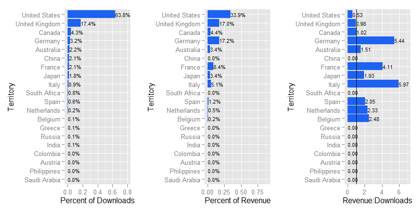
This R code reads in the downloads report and the revenue report, reformats the data so that it can be plotted, merges the data by territory, and creates three different plots. These plots show you which territories generate what percent of your total downloads, which territories generate what percent of your total revenue, and which territories generate the most revenue per downlod.

Reading the Data

The first step is to actually read your reports data into R. First, just save your filenames and file paths as variables to make it a little easier to swap out which reports your are using.

directory <- paste(getwd())

rev.filename <- "Sample-intlRevenue-AppAnnieFormat.csv"
DL.filename <- "Sample-intlDownloads-AppAnnieFormat.csv"

The getData function will read the files into R and process them appropriately. It works as follows:

Read the App Annie report into R
Sum the total downloads or revenues for each territory for the time period of the report
Return properly-formatted summary data

Then run the getData function on both reports.

getData <- function(directory,filename,type){
      
      #read the .csv file into R and skip header information
      if (type == "Revenue"){
            df <- read.csv(paste(directory,'/',filename,sep=""), skip=9)     
      } else if (type == "Downloads") {
            df <- read.csv(paste(directory,'/',filename,sep=""),skip=8)     
      } else {print("Please specify type as either 'Revenue' or 'Downloads'")}
      
      #take on the territory lables and the totals by territory
      df <- df[c(1,nrow(df)),3:ncol(df)-1]
      
      #transpose the data
      df <- as.data.frame(t(df))
      
      #fix row names     
      if (type == "Revenue"){
            colnames(df)[1:2] <- c("Territory","Revenue")
      } else {
            colnames(df)[1:2] <- c("Territory","Downloads")
      }     
      df       
}

#run the get data function to get the download and revenue data
rev.data <- getData(directory,rev.filename,'Revenue')
DL.data <- getData(directory,DL.filename,'Downloads')

Processsing the Data

At this point, the revenue and the downloads data are still in separate data frames. Combine them like this:

#join the data frames based on territories
both.data <- merge(x=DL.data, y=rev.data, by='Territory', all.x=TRUE)
rm(rev.data)
rm(DL.data)

#set column classes to numeric
both.data$Revenue <- as.numeric(as.character(both.data$Revenue))
both.data$Downloads <- as.numeric(as.character(both.data$Downloads))

#replace NAs with 0s (Necessary to show which territories
# have DL's but no revenue)
both.data$Revenue[is.na(both.data$Revenue)] <- 0

Since we want to compare which territories generated what percentage of total downloads and revenue, add those metrics as two new columns.

#add percent of total columns
both.data$PercentTotalRev <- both.data$Revenue / sum(both.data$Revenue)
both.data$PercentTotalDL <- both.data$Downloads / sum(both.data$Downloads)

Since these reports include 150+ territories by default, and most of them will have zero information, just select the top 20 by downloads.

#order the data by downloads and select top 20
require(sqldf)
both.data <- sqldf("
                   SELECT *
                   FROM 'both.data'
                   ORDER BY Downloads DESC")

both.data <- both.data[1:20,]

Finally, in order to compare the relative value of each download for each territory, perform that calculation and add it as a new column.

#add relative download value ratio column
both.data$Ratio <- both.data$PercentTotalRev / both.data$PercentTotalDL

###Plotting the Comparisons

The data is now all in one data frame and is formatted properly. It’s ready to plot. Depending on your data, you might want to adjust the scales.

#ggplot reverts to ordering territories alphabetically unless we explicitly set the order of the factors
both.data$Territory <- factor(both.data$Territory, levels = both.data$Territory[order(both.data$Downloads)])

#ratio plot
require(ggplot2)
require(scales)
plot1 <- ggplot(both.data,aes(x=Territory,y=Ratio))+ geom_bar(stat="identity",fill="#1D62F0")
plot1 <- plot1 + coord_flip() + geom_text(aes(label=format(round(Ratio,2),nsmall=2)),size=3,hjust=0)
plot1 <- plot1 + ylab('Revenue:Downloads')
plot1 <- plot1 + scale_y_continuous(limits=c(0,7)) + geom_hline(yintercept=1)
plot1

#downloads plot
plot2 <- ggplot(both.data,aes(x=Territory,y=PercentTotalDL))+ geom_bar(stat="identity",fill="#1D62F0")
plot2 <- plot2 + coord_flip() + geom_text(aes(label=percent(PercentTotalDL)),size=3,hjust=0)
plot2 <- plot2 + ylab('Percent of Downloads')
plot2 <- plot2 + scale_y_continuous(limits=c(0,.8)) 
plot2

#revenue plot
plot3 <- ggplot(both.data,aes(x=Territory,y=PercentTotalRev))+ geom_bar(stat="identity",fill="#1D62F0")
plot3 <- plot3 + coord_flip() + geom_text(aes(label=percent(PercentTotalRev)),size=3,hjust=0)
plot3 <- plot3 + ylab('Percent of Revenue')
plot3 <- plot3 + scale_y_continuous(limits=c(0,.9)) 
plot3

The gridExtra library provides easy functionality to put these three plots into one figure.

#multiplot
library(gridExtra)
grid.arrange(plot2,plot3,plot1,ncol=3)