Where Should You Spring Ski? How to use the powderlin.es API and R to Make Better Decisions
14 May 2015
Eric Fram
All of the code used here is available on GitHub
##Introduction
If you like to get the most out of every ski season, you’ve probably found yourself booking trips right before resorts close for the spring (April 1 to April 15-ish). So late in the year though, it can be hard to tell ahead of time which resorts will have enough snow to make a trip worthwhile.
If this is an issue you’ve run into, then this analysis might be able to help you.
The R code we use here reads historical snow data for a selection of ski areas from the powderlin.es API, then performs several different analyses in order to create a useful model for predicting which resorts will have the deepest snow during a given period.
###A few caveats
The data from the powderlin.es API is from Natural Resource Convervation Services SNOTEL (Snow Telemetry) stations. SNOTEL stations measure snow depth accurately, but aren’t typically located on ski slopes. Thus, the SNOTEL data differs somewhat from the on-slope snow depth reported by resorts. Another issue is that not all major ski resorts have a SNOTEL station nearby (such as Aspen and Park City), so data for those areas is not available through this API.
I’ve chosen to use powderline.es for this first iteration as it is free and does not require authentication. Data provided directly by ski resorts, such as that provided through the OnTheSnow API will better reflect actual ski conditions, but those typically require authentication and/or payment.
Using ski resort snow data instead of SNOTEL data is at the top of the to do list for the next iteration of this program.
##Getting the Data
###Retrieving SNOTEL Station ID’s
In order to retrieve historical snow depth data from the powederlin.es API, we have to know the 3-part station ID for each area we want to compare. The code here takes the names of the stations and looks up their station ID. It then saves all of the station names and station IDs into a data frame which we later use to lookup the ID’s by name.
The code will accept any number of station names as long as the names match those in the SNOTEL network. I’ve picked 5 examples here.
names <- c("BRIGHTON","SNOWBIRD","VAIL MOUNTAIN","SQUAW VALLEY G.C.","TAOS POWDERHORN")


      #Function to lookup what stations correspond to what ID numbers
      stationsLookup <- function(name){
            require(RJSONIO)
            require(jsonlite)

            #URL for stations list as a variable
            stationsURL <- "http://api.powderlin.es/stations"

            #Read the JSON and make a data frame
            stationsRaw <- readLines(stationsURL)
            stationsJSON <- fromJSON(stationsRaw)

            do.call("rbind",stationsJSON)
            rm(stationsRaw)

            stationID <- stationsJSON$triplet[which(stationsJSON$name==name)]
      }

      #loop through the selected resorts and get their SNOTEL ID's
      ids <- c()
      for (i in 1:length(names)){
            ids[i] <- stationsLookup(names[i])
      }

      #save resort names and IDs in a new data frame
      lookup <- data.frame(names,ids)
      rm(names)
      rm(ids)
###Retrieving historical snow data
Now that we have the station ID’s for the areas we are interested in, we can retrive the historical snow depth data for each station. Here, we’re interested in data for the first two weeks in April of 2015.
This code gets the historical snow depth data for the selected stations across the selected date range.
startDate <- "2015-4-01"
endDate <- "2015-4-15"

 #function to lookup the amount of snow for each day during the selected date range
      snowLookup <- function(startDate, endDate, stationID) {

            require(RJSONIO)
            require(jsonlite)

            infoURL <- paste("http://api.powderlin.es/station/",stationID,"?start_date=",startDate,
                             "&end_date=",endDate,sep='')

            infoRaw <- readLines(infoURL)

            infoJSON <- fromJSON(infoRaw)

            rm(infoRaw)

            info <- data.frame(infoJSON$data["Date"],infoJSON$data["Snow Depth (in)"],
                               lookup$names[which(lookup$ids==stationID)])
            info
      }

      #loop over the selected resorts using snowLevels to get the snow depth on each date in the date range
      #save all of the resort data in a single data frame
      combined <- data.frame()
      for (i in 1:nrow(lookup)){
            df <- snowLookup(startDate,endDate,as.character(lookup$ids[i]))
            combined <- rbind(combined,df)
            combined
      }

      #fix column names
      colnames(combined) <- c("Date","SnowDepth","Resort")
      combined$Date <- as.POSIXct(combined$Date)
      combined$SnowDepth <- as.numeric(as.character(combined$SnowDepth))
      combined
###Putting It Together
To make thing easier on ourselves going forward, I’ve combined all of the code shown so far into a single function called snowData that gets the station ID’s for each station name that you select, then gets historical snow data for the range of dates that you select, then returns all the data in a single data frame.
snowData <- function(startDate,endDate,names){

      require(RJSONIO)
      require(jsonlite)

      #Function to lookup what stations correspond to what ID numbers
      stationsLookup <- function(name){
            #URL for stations list as a variable
            stationsURL <- "http://api.powderlin.es/stations"

            #Read the JSON and make a data frame
            stationsRaw <- readLines(stationsURL)
            stationsJSON <- fromJSON(stationsRaw)

            do.call("rbind",stationsJSON)
            rm(stationsRaw)

            stationID <- stationsJSON$triplet[which(stationsJSON$name==name)]
      }

      #loop through the selected resorts and get their SNOTEL ID's
      ids <- c()
      for (i in 1:length(names)){
            ids[i] <- stationsLookup(names[i])
      }

      #save resort names and IDs in a new data frame
      lookup <- data.frame(names,ids)
      rm(names)
      rm(ids)

      #function to lookup the amount of snow for each day during the selected date range
      snowLookup <- function(startDate, endDate, stationID) {

            infoURL <- paste("http://api.powderlin.es/station/",stationID,"?start_date=",startDate,
                             "&end_date=",endDate,sep='')

            infoRaw <- readLines(infoURL)

            infoJSON <- fromJSON(infoRaw)

            rm(infoRaw)

            info <- data.frame(infoJSON$data["Date"],infoJSON$data["Snow Depth (in)"],
                               lookup$names[which(lookup$ids==stationID)])
            info
      }

      #loop over the selected resorts using snowLevels to get the snow depth on each date in the date range
      #save all of the resort data in a single data frame
      combined <- data.frame()
      for (i in 1:nrow(lookup)){
            df <- snowLookup(startDate,endDate,as.character(lookup$ids[i]))
            combined <- rbind(combined,df)
            combined
      }

      #fix column names
      colnames(combined) <- c("Date","SnowDepth","Resort")
      combined$Date <- as.POSIXct(combined$Date)
      combined$SnowDepth <- as.numeric(as.character(combined$SnowDepth))
      combined
}
We can run the snowData function and save the results as so.
startDate <- "2015-4-01"
endDate <- "2015-4-15"
names <- c("BRIGHTON","SNOWBIRD","VAIL MOUNTAIN","SQUAW VALLEY G.C.","TAOS POWDERHORN")

combined <- snowData(startDate,endDate,names)
head(combined)
##         Date SnowDepth   Resort
## 1 2015-04-01        18 BRIGHTON
## 2 2015-04-02        18 BRIGHTON
## 3 2015-04-03        20 BRIGHTON
## 4 2015-04-04        18 BRIGHTON
## 5 2015-04-05        17 BRIGHTON
## 6 2015-04-06        16 BRIGHTON
##Analyzing the Data
The data we get from the snowData function allows us to compare snow depth between resorts for a single period. We can graph the data frame as-is.
require(ggplot2)
require(scales)
plot <- ggplot(combined,aes(x=Date,y=SnowDepth,color=Resort,group=Resort))
plot <- plot + geom_line(stat='identity') + ylab('Snow Depth (Inches)')
plot <- plot + geom_point(stat='identity')
plot <- plot + scale_x_datetime(breaks='1 day',labels=date_format('%m-%d-%Y'))
plot <- plot + scale_y_continuous(limits=c(0,60))
plot <- plot + theme(axis.text=element_text(size=8))
plot
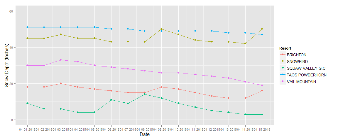
This chart is useful to see which areas had the most snow for spring skiing this year, but doesn’t have much predictive value.
###Get Several Years of Data
To help us predict which resorts on average have the most snow during our date range, we should get a few years of data. I’m only going back to 2012 here, as SNOTEL snow depth data doesn’t go back much farther than that for most stations. In future versions, where we use a different API, we will be able to get data from farther back (hopefully)
This code will get data for a group of date ranges.
#combine the data for several years into one DF
startDates <- c("2012-4-01","2013-4-01","2014-4-01","2015-4-01")
endDates <- c("2012-4-15","2013-4-15","2014-4-15","2015-4-15")

for (i in 1:length(startDates)){
      df <- snowData(startDates[i],endDates[i],names)
      combined <- rbind(combined,df)
}
###Analysis 1 - Try to Predict Snow Depth Assuming Little Year-to-Year Variance
As a first attempt, let’s try to create a snow-depth prediction model assuming that the conditions in April for each area aren’t all that different from year to year (which is really not a very good assumption). We will compare all of the data points we have between days in April, but not across years.
#save a copy of these date for different analysis
stretched <- combined

#remove year information
combined$Date <- as.numeric(substr(combined$Date,nchar(combined$Date)-1,nchar(combined$Date)))

#plot new data
require(ggplot2)
require(scales)
plot2 <- ggplot(combined,aes(x=Date,y=SnowDepth,color=Resort,group=Resort))
plot2 <- plot2 + ylab("Snow Depth (Inches)") + xlab("Day in April")
plot2 <- plot2 + geom_point(size=3)
plot2
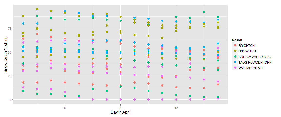
At a glance, it doesn’t look like we will be able to fit a model to this data, but let’s give it a try anyways.
#see if we can fit a linear model to each resort to predict what the snow depth will be
require(lme4)
fit <- lmList(SnowDepth ~ Date | Resort, data=combined)
summary(fit, pool=FALSE)
## Call:
##   Model: SnowDepth ~ Date | NULL
##    Data: combined
##
## Coefficients:
##    (Intercept)
##                   Estimate Std. Error   t value     Pr(>|t|)
## BRIGHTON          35.28952   4.068301  8.674265 7.609110e-13
## SNOWBIRD          64.62095   4.136574 15.621853 5.551468e-25
## SQUAW VALLEY G.C. 42.62667   7.262994  5.869022 1.194594e-07
## TAOS POWDERHORN   59.67429   3.453493 17.279401 1.657122e-27
## VAIL MOUNTAIN     35.15429   4.455624  7.889869 2.267306e-11
##    Date
##                      Estimate Std. Error    t value  Pr(>|t|)
## BRIGHTON          -0.38285714  0.4474535 -0.8556356 0.3949991
## SNOWBIRD          -0.05928571  0.4549625 -0.1303090 0.8966804
## SQUAW VALLEY G.C. -0.55000000  0.7988228 -0.6885131 0.4933120
## TAOS POWDERHORN   -0.13428571  0.3798335 -0.3535383 0.7247039
## VAIL MOUNTAIN     -0.59428571  0.4900533 -1.2126962 0.2291559
| A p-value (Pr(> | t | for the slope) of <0.05 would tell us that a model is useful. All of these are way above that. These models don’t have predictive value. Let’s try something else. |
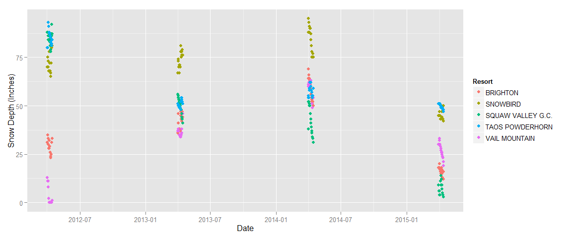
###Analysis 2 - Try to Predict Snow Depth Allowing for Year-to-Year Changes
Instead of plotting several years data by day in April, let’s keep it spread out across time.
#check to see trends over time
plot4 <- ggplot(stretched,aes(x=Date,y=SnowDepth,color=Resort,group=Resort))
plot4 <- plot4 + ylab("Snow Depth (Inches)") + xlab("Date")
plot4 <- plot4 + geom_point(stat='identity') #+ geom_line(stat='identity')
plot4
Now, let’s see if we can fit linear models to the data.
#see if we can fit a linear model over time to predict what snow depth will be
require(lme4)
fit <- lmList(SnowDepth ~ Date | Resort, data=stretched)
summary(fit, pool=FALSE)
## Call:
##   Model: SnowDepth ~ Date | NULL
##    Data: stretched
##
## Coefficients:
##    (Intercept)
##                    Estimate Std. Error   t value     Pr(>|t|)
## BRIGHTON           264.8207   68.25552  3.879843 2.268854e-04
## SNOWBIRD           483.4662   55.84583  8.657159 8.193498e-13
## SQUAW VALLEY G.C. 1123.9783   31.49328 35.689469 5.929392e-48
## TAOS POWDERHORN    475.1044   38.48937 12.343782 1.519527e-19
## VAIL MOUNTAIN     -234.4644   74.70531 -3.138523 2.449863e-03
##    Date
##                        Estimate   Std. Error    t value     Pr(>|t|)
## BRIGHTON          -1.672577e-07 4.906518e-08  -3.408888 1.065197e-03
## SNOWBIRD          -3.015314e-07 4.014452e-08  -7.511146 1.162631e-10
## SQUAW VALLEY G.C. -7.807606e-07 2.263880e-08 -34.487720 6.294047e-47
## TAOS POWDERHORN   -2.995070e-07 2.766791e-08 -10.825067 7.798340e-17
## VAIL MOUNTAIN      1.904631e-07 5.370158e-08   3.546695 6.857590e-04
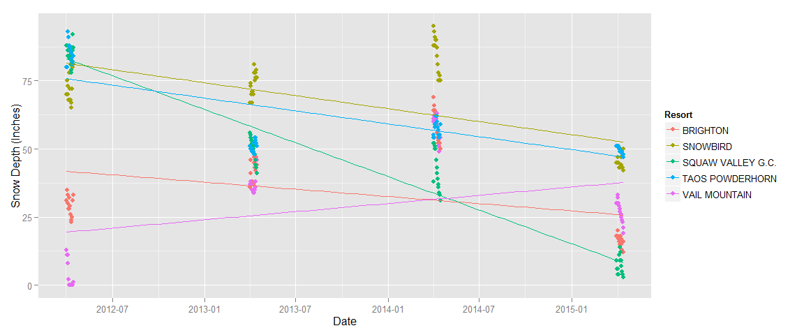
It looks like we can! These models will only work for predicting snow in the first two weeks of April, but that’s what we want. Let’s add these models to the plot to see what they look like.
plot4 <- plot4 + stat_smooth(aes(group=Resort),method='lm',se=FALSE)
plot4
Now, let’s use these models to see how accurately they would have predicting snow depth for April 2015 (data we actually have)
#see how well the model predicts the data we actually have
predictionDate <- "2015-4-1 PDT"
predictionData <- data.frame(Resort = NA, fit = NA, lwr = NA, upr = NA)

for (i in 1:length(names)) {
      fitPredict <- lm(SnowDepth ~ Date, data= stretched[which(stretched$Resort==names[i]),])
      newdata <- data.frame(Date = as.POSIXlt(predictionDate))
      predictionData[i,] <- c(names[i],predict(fitPredict,newdata,interval='predict', level=.95))
}

print(predictionData)
##              Resort              fit               lwr              upr
## 1          BRIGHTON 25.9982586418548 -5.56593742467681 57.5624547083865
## 2          SNOWBIRD 52.9181214121292   27.092685993546 78.7435568307125
## 3     VAIL MOUNTAIN 37.4925423554214  2.94569727130131 72.0393874395415
## 4 SQUAW VALLEY G.C. 9.15239013957171 -5.41141247850187 23.7161927576453
## 5   TAOS POWDERHORN 47.4468381609008   29.647750184776 65.2459261370257
Not so terrible. Our confidence intervals are really wide, but we can at least get some idea of which areas are better than others for spring skiing.
Now, let’s predict what the snow depth will be next April.
#predict future snow levels using linear model
predictionDate <- "2016-4-1 PDT"
predictionData <- data.frame(Resort = NA, fit = NA, lwr = NA, upr = NA)

for (i in 1:length(names)) {
      fitPredict <- lm(SnowDepth ~ Date, data= stretched[which(stretched$Resort==names[i]),])
      newdata <- data.frame(Date = as.POSIXlt(predictionDate))
      predictionData[i,] <- c(names[i],predict(fitPredict,newdata,interval='predict', level=.95))
}

print(predictionData)
##              Resort               fit               lwr                upr
## 1          BRIGHTON  20.7091696927108 -11.3592085895874   52.7775479750089
## 2          SNOWBIRD  43.3829762539839   17.145025172875   69.6209273350929
## 3     VAIL MOUNTAIN  43.5154437523685  8.41677390877921   78.6141135959578
## 4 SQUAW VALLEY G.C. -15.5371347071027 -30.3335683181688 -0.740701096036675
## 5   TAOS POWDERHORN  37.9757076896473  19.8923107580366   56.0591046212579
Based on this, it looks like Snowbird and Vail are the winners.
##Discussion
This is just a first iteration of this analysis. As I mentioned before, the limitations of the SNOTEL data reduce the predictive value of these models. Not only do we have access to just a few years worth of snow depth data, but the SNOTEL readings are not necessarily representative of actual skiing conditions. This is especially obvious in the case of Brighton: the SNOTEL readings show less than 25 inches of base depth, while readings on the mountain show more than 50 inches. Using OnTheSnow or similar data will allow us to develop more useful models, since the ski conditions on the actual slopes are what we are interested in.
Secondly, year-over-year weather patterns are affected by things such as El Nino/a cycles and climate change, so using a linear model to predict snow depth more than a year in future is probably not going to work very well. I will begin to explore ways to potentially account for this.